Clouds are not spheres, coastlines are not circles,mountains are not cones and bark is not smooth. it was famous sentence from mandelbrot. we need to spicial geometry and spicial dimension for presentation of nature. we also need to new dimension over of ordinery dimension (0,1,2,3 for point , line , surface and volum). so it may be variaty and decimal. we can see dimensions for example (( 0,63)) ,((1,7)),((2,3)), ((3,2)).cantor set dimension as a dust is equal ((0,63)) , dimension of serpinski triangular is ((1,58)) .Draw an equilateral triangle with sides of 2 triangle lengths each Connect the midpoints of each side. How many equilateral triangles do you now have? Shade out the triangle in the center. Think of this as cutting a hole in the triangle Draw another equilateral triangle with sides of 4 triangle lengths each. Connect the midpoints of the sides and shade the triangle in the center as before. Draw another equilateral triangle with sides of 4 triangle lengths each. Connect the midpoints of the sides and shade the triangle in the center as before. Notice the three small triangles that also need to be shaded out in each of the three triangles on each corner - three more holes. Draw an equilateral triangle with sides of 8 triangle lengths each. Follow the same procedure as before, making sure to follow the shading pattern. You will have 1 large, 3 medium, and 9 small triangles shaded. How about doing this one on a poster board? Follow the above pattern and complete the Sierpinski Triangle. Use your artistic creativity and shade the triangles in interesting color patterns. Does your figure look like this one? Then you are correct!

Dimension of river networks is varied between 1.6 to 1.8 but it will never be equal to 2 because there is no river networks in nature which to be space filling. Fractal dimension of Topography surfaces is 2.43 in Alps Mountains (in mononfractal state). i will represente some concepts of fractal like, self similarity , self-affinity , and fractal geometry:
A curve can be space filling so that fractal dimension of this curve will be 2 . it means that fractal dimension of curve will be equal to Euclidean Dimension of surface. Peano curve is good example so that its dimension is 2 . First time Weierstrass introduced Continuous Non-Differentiable Function. The function has the property that it is continuous everywhere but differentiable nowhere. this link is example of space filling curve:
http://www.physics.mcgill.ca/~gang/multifrac/intro/intro.htm
Most of papers in mathematic are about pure mathematical self-similarity but not self-affinity. A self-similar object is exactly or approximately similar to a part of itself, i.e., the whole has the same shape as one or more of the parts. A self-affinity is a fractal whose pieces are scaled by different amounts in the x- and y-directions. the self-similar is isotropy and self-affine is anisotropy.drainage basin , individual stream , braided river are self-affine. sapozhnikov et al (1993) demonestrated that natural and simulated individual stream show a complicated geometry: self-similarity at small scales and self-affinity at larger scales. self-affine behavior of the streams caused by gravity which makes the stream scale differently in the direction of the mainstream slope and in the prependicular direction. self-affinity in natural river courses was also reported by Ijjasz-Vasquez et al. (1994). Anisotropic spatial scaling(external scaling) was revealed in simulated river networks . it is shown that the rivers exhibit anisotropy scaling (self-affinity) with fractal exponents Vx = 0.72-0.74 and Vy = 0.51-0.52 the x axis being oriented along the river and the y axis in the perpendicular direction. you can find mathematical self-similarity and self-similarity in the nature in follow link:
http://local.wasp.uwa.edu.au/~pbourke/fractals/selfsimilar//
I will discuss about fractal dimension in river network and topography
statistical self similarity:
River networks are statistical self-similarity . It means that all fractal laws establish on mean of parameter (mean of length, area, etc). statistic of parameter have fractal behavior not exactly.
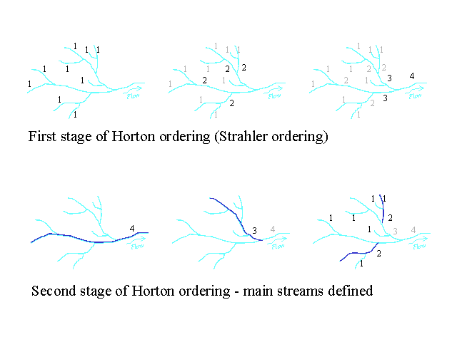
Horton ordering system:
Horton’s ordering method operates in two stages, as shown in Figure 5. In the first step, the unbranching streams are removed and numbered as one, these process is then repeated, incrementing the number each time, until the entire network has been ordered. This method is also known as the Strahler ordering. In the second stage, a main stream is selected, and assigned the highest order occurring on it throughout its length. Of the remaining tributaries, a main stream is selected in each, and assigned the maximum order which occurs on its length. This process continues until all components have been assigned an order in the second method [Goudie 1985]. click on the figure
Tokunaga ordering system:
Scheidegger (1968) proposed the following definition of a cyclic system: a drainage network is said to be cyclic if each cycle (referring to particular system order) is entirely similar to the previous and following cycles, in which new parts of the network are created with same bifurcation ratio. This cyclic model has been shown to hold only for the structurally Hortonian network (scheidegger, 1968, 1970; Tokunaga, 1978). Tokunaga (1978) revised the concept of scheidegger’s cyclic net by removing the restriction on the bifurcation ratio. This allows the defination of more general cyclic systems for the discription of the drainage basin. However without the restriction on the bifurcation ratio the cycicity definition becomes ambiguous because there is no clear way establishing how the previous and following cycles are entirely similar. To remove this ambiguity, the Tokunaga cyclic network is defined as follows: A drainage network is said to be cyclic if the sequence of the number of tributaries of order lamda,lamda=1,...,omega-1, entering each omega^th order stream follows a geometric series . The configuration of trees considered here is topologically independent of tributaries entering from the left or right sides having different ordering. The topological configuration of a Tokunaga cyclic tree is determined by two parameters, ((ٍٍEpsilon)) and ((K)). Let the number of streams of order i flowing laterally into the higher order stream of order j be denoted jei (Tokunaga, 1978). Tokunaga suggests that jej-k (k>0) are on average independent of j, denoted:
This is self-similarity property. Furthermore Tokunaga suggests that analogous to Horton’s ratio the E, K are also geometrically to dependent on order.
K=Ek/Ek-1
The two parameter E1 and K are analogous to Rb in that they completely describe the network branching structure. The Number of streams of each order Omega (uppercase) within a basin of order Omega (dawn case) is (Tokunaga,1978,2003;Tarboton,1996)

where P and Q are parameters given by

Putting E1=Rb-2 and k=0 one obtains P=0, Q=Rb and (omega = w) N (W, w) ^W-w =Rb^W-w thus Tokunaga cyclicity generalizes Horton’s bifurcation law, retaining it as a special case (Tarboton, 1996). To calculate similarity dimensions for a Tokunaga network of order W, let the linear scale reduction factor for each order be r (1/RL) for streams. The network is comprised of 2+E1 sub networks order Reduced by factor r^2, E1K^2 network order W-3 reduced by factor r^3 and so on. The self-similarity mention is then calculated using uneven scale ratios (Mandelbrot, 1983; Tarboton, 1996).
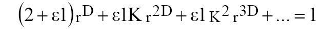
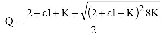
This geometry series can be reduced to a quadratic equation for r^-D large root gives.
Db= lnQ/ln (1/r)
which for stream lengths (r=1/RL) gives
Db=lnQ/lnRL
figure 8.6: fractal tree in order Tokunaga ordering system (Ref. Turcotte,1997) click on the figure

Tokunaga's parameters have deviation in real river. Tokunaga(1978) suggested this deviation depends on the size of network magnitude and assumed the deviation would diminish as basin order increased .Peckham (1995) has determined the branching-ratio matrices for the Kentucky River basin in Kentucky and the Powder River basin in Wyoming, Both river basins are eighth order, with the Kentucky River basin having an area of 13,500 km2 and the Powder River basin an area of 20,181 km2. For the Kentucky River basin, the bifurcation ratio is Rb = 4.6, the length-order ratio is Rr = 2.5, and the fractal dimension is D = 1.67; for the Powder River basin the bifurcation ratio is Rb = 4.7, the length-order ratio is Rr = 2.4, and the fractal dimension is D = 1.77. Scott Peckham (1995a) presents a number of ideas on statistically self-similar topologies. Peckham(1995b) first suggested that ramdom self-similar trees could be generated using a sampling process from random distribution. He rejected Tokunaga canjactur by analysis of large river basin.Cui(1999) used Stochastic Tokunaga Model in karuah river . He compared his result with Peckham's data from Kentucky and Tarboton's data from buck creek. stochastic Tokunaga model is generalisation of Tokunaga cyclic model that describes average network topology. The stochastic model assumes that actual tributary numbers are random realisations from a negative binomial distribution whose mean is defined by Tokunaga parameters epsilon and K. this parameters can be interpreted as representing the effects of regional controls. Upon these regional controls is superimposed an inherent spatial variability in network topology. a third parameter alpha characterises this spatial variability. when alpha becomes large, the negative binomial model degenerates to a poisson model. Cui (1999) used Mont Carlo Bayesian methods for evaluate the uncerttainity in Tokunaga parameters and in stream number related statistics such as stream numbers and biurcation ratio. he noticed that the tributary data for an order-5 fails to identify the Tokunaga parameters, whereas data from order-6 and 8 basins yields relatively precise inferenc. he also found that the information in low order networks provides little power for discriminating between model hypotheses.
Multifractal and topography ( Universal Multifractal ):
( These are abstracts of Kravchenko, lovejoy, Tennekoon et al 's articles)
((A single fractal dimension might not always be sufficient to represent complex and heterogeneous behavior of topography spatial variations. A recently developed extension of the monofractal approach describes the data with a set of fractal, (Mandelbrot, 1974), instead of a single value. This set is called a multifractal spectrum and the method of variability characterization based on the multifractal spectrum is referred to as a multifractal analysis (Frisch and Parisi, 1985). The multifractal approach implies that a statistically self-similar measure can be represented as a combination of interwoven fractal sets with corresponding scaling exponents. A combination of all the fractal sets produces a multifractal spectrum that characterizes variability and heterogeneity of the studied variable. The advantage of the multifractal approach is that the multifractal parameters can be independent of the size of the studied objects (Cox and Wang, 1993), as well as that no assumption is required about the data following any specific distribution(Scheuring and Riedi, 1994).
The Schertzer and Lovejoy (1987) have shown topography as multifractal model. Scherzer and Lovejoy (S&L) model is generalization of the lognormal model (Kolmogrov, 1962; Obukov, 1962; Yaglom, 1966). It is relies on using the alpha-stable family distribution, which is generalization of Gaussian distribution, to include, for example, infinite variance distributions. The alpha-stable distribution depends on four parameters (Uchaikin and Zolotorev, 1999), but in multifractal studies two of the parameters are fixed (Boufadel et al.2000). Hence, only two parameters are of interest: alpha and c1. The parameter c1 is such 0 the upper limit being the Gaussian distribution. As alpha decreases, the frequency of sudden large jumps in the random field increases. The parameter c1 is known as the scale parameter. It is measure of width of distribution, and is equal to half the variance when alpha=2. As c1 increases, the magnitude of the sudden large jumps increases (Boufadel et al, 2000).studies have shown that the S&L model is flexible in fitting observed data. It has been shown that, for canonical processes, universality class exists which means that it may be expectedk(q) to be given by following functional form (lavalee,1991;Tnnekoon et al,2003):))
.1.jpg)
Where C1 and alpha(0= are the fundamental parameters needed to characterize the processes. The Lévy index alpha indicates the class to which the probability distribution belongs; it tells us how far we are from monofractality: alpha=0 corresponds to monofractalbeta model; alpha=2 is the maximum. The above functions are for conserved (stationary) quantities and are multiplicative analogs of the standard central limit theorem for the addition of random variable. Closer analysis shows that there are actually five qualitatively different cases for Lévy index alpha (lavallée et al, 1993).
Shaun Lovejoy homepage and multifractal :
http://www.physics.mcgill.ca/~gang/Lovejoy.htm
http://www.physics.mcgill.ca/~gang/multifrac/intro/intro.htm
I think that if Topography is multifractal spectrum then gradiant of slopes will be multifractal .in the other hand some researcher argued that Topography's gradients have fuzzy behaviour. I have nice idea . I conjacture that gradiant of slopes are Fuzzy -Multifractal. I suggest and invite some scintists for study about Fuzzy- Multifractal .
1 : professor shaon Lovejoy from Mcgill university:
http://www.physics.mcgill.ca/~gang/Lovejoy.htm
2 :professor Eiji Tokunaga from Chuo University, Hachioji-shi, Tokyo , Japan (tokusan@tamacc.chuo-U.ac.jp)
3 :Angela M. Coxe
http://www.lafayette.edu/news.php/view/2716
(email: coxea@lafayette.edu)
4 :professor Clifford Reiter , Professor of Mathematics from Lafayette
http://lafayette.edu/news.php/view/6753/
/ww2.lafayette.edu/~reiterc/index.html
( reiterc@lafayette.edu )
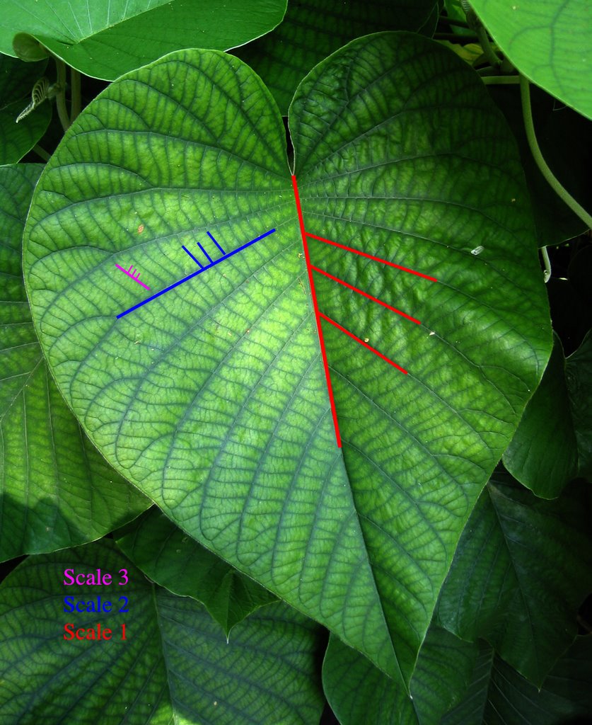
Nature is fuzzy and multifractal :
http://ramin-parhizi.magix.net/
fuzzy-multifractally leaf:

and fuzzy fractally leaf again:

Tokonaga (2003) explained fractal theory in drainage basin and made a 2 dimensinal serpinsky space. He established area interbasin law : click on the figure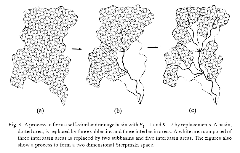
Inner Product Fractals from Fuzzy Logics : (Angela M. Coxe )
(email: coxea@lafayette.edu)

http://www.vector.org.uk/archive/v192/coxe192.htm
and Tokunaga again :

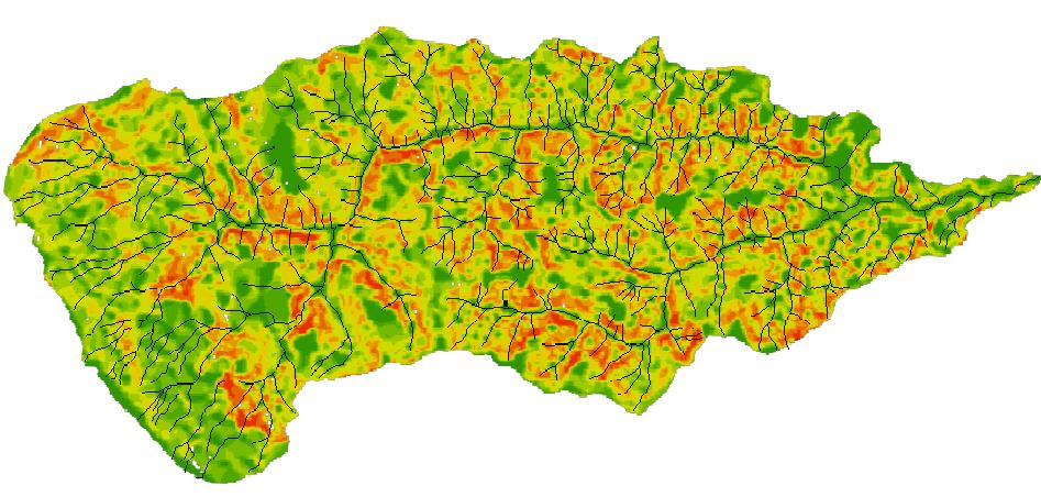
gradient of Topography in Shafaroud drainage basin : click on the picture. follow image extracted from topography rectified contour map by Arcgis 8,3 . some inner peaks have not been entered. it will be cause that inner peaks to be as plan surface.